Physical Address
304 North Cardinal St.
Dorchester Center, MA 02124
Physical Address
304 North Cardinal St.
Dorchester Center, MA 02124
→ Step-by-step guide for training YOLO-NAS object detection models in PyTorch using custom datasets.
Every year, new YOLO versions are published, and last I saw, there was something like YOLOv12. If you have used YOLO models before, you probably used models like YOLOv5, YOLOv8, or something like YOLOv{some number}.
There are different YOLO models you probably haven’t heard about or have heard but haven’t used, like YOLOX and YOLO-NAS. Now, I will share with you my pipeline to train custom YOLO-NAS models and how to make predictions with the trained model.

YOLO-NAS has an important advantage compared to other YOLO variants, and it is licensing. If you are planning to use your YOLO model commercially, YOLO-NAS might be a good choice. I don’t want to give misinformation, but I know it has advantages. For better information, you can visit its Github page.
Also, I have a YouTube video about this article, you can watch it.
Now, I will train a model to show how the pipeline works. I chose a small dataset from Roboflow. You can randomly choose any dataset and follow this pipeline because the steps are the same. If you want to use this code exactly, don’t forget to export the dataset in YOLO format. You can use different formats like COCO, but you need to change some parts at the beginning when preparing the data.
I have a GPU supported PyTorch environment, and I will train my model locally on my computer. If you don’t have a GPU supported environment, you can use Kaggle or Google Colab, it will save a huge amount of time for you.
If you want to create a GPU-supported PyTorch environment, you can watch this video.
There are 6 main steps:
!pip install super_gradients
import torch
import os

# Check if GPU is available
DEVICE = 'cuda' if torch.cuda.is_available() else "cpu"

# current directory
HOME = os.getcwd()
EXPERIMENT_NAME="yolonas-m-model-1-20epoch"
CHECKPOINT_DIR = f'{HOME}/checkpoints'
Initialize the Trainer object and create dataset parameters. You need to set the paths for the dataset and set class names of model.
from super_gradients.training import Trainer

"""
Trainer --> Initialize the Trainer for the YOLO-NAS model
Trainer is responsible for managing the training process, including data loading, model training, and evaluation.
trainer is an instance of the Trainer class from the super_gradients.training module.
"""
trainer = Trainer(experiment_name=EXPERIMENT_NAME, ckpt_root_dir=CHECKPOINT_DIR)


# Dataset , Label information
dataset_params = {
    'data_dir': "C:/ml_dl_cv_files/ObjectDetection-Yolo-TF-Models/Custom-YOLONAS-model/dataset",
    'train_images_dir':'train/images',
    'train_labels_dir':'train/labels',
    'val_images_dir':'valid/images',
    'val_labels_dir':'valid/labels',5
    'classes': ['player', 'referree', 'football'] # labels here
}
from super_gradients.training.dataloaders.dataloaders import (
    coco_detection_yolo_format_train, coco_detection_yolo_format_val)

# you can increase this number depending on your GPU, more batch size means faster training
BATCH_SIZE = 4

train_data = coco_detection_yolo_format_train(
    dataset_params={
        'data_dir': dataset_params['data_dir'],
        'images_dir': dataset_params['train_images_dir'],
        'labels_dir': dataset_params['train_labels_dir'],
        'classes': dataset_params['classes']
    },
    dataloader_params={
        'batch_size': BATCH_SIZE,
        'num_workers': 2
    }
)

val_data = coco_detection_yolo_format_val(
    dataset_params={
        'data_dir': dataset_params['data_dir'],
        'images_dir': dataset_params['val_images_dir'],
        'labels_dir': dataset_params['val_labels_dir'],
        'classes': dataset_params['classes']
    },
    dataloader_params={
        'batch_size': BATCH_SIZE,
        'num_workers': 2
    }
)
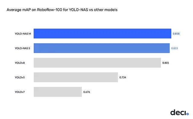
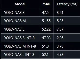
In general, larger models give more accuracy, but they work slower than light models.
I will use the YOLO-NAS M model; you can choose whichever model you want. If you follow this pipeline, it will work without any problem.
from super_gradients.training import models

MODEL_ARCH = "yolo_nas_m"

model = models.get(
    MODEL_ARCH,  # yolo_nas_m
    num_classes=len(dataset_params['classes']),
    pretrained_weights="coco"
)
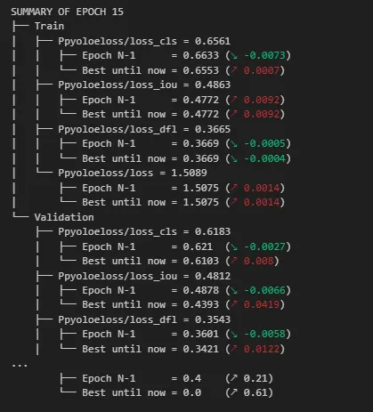
Decide on the training parameters (I set mixed_precision to False because it was causing the model metrics to be NaN, and it was probably because my GPU’s memory is 6GB, which is not enough. Depending on your GPU, you can set ‘mixed_precision’ to True).
from super_gradients.training.losses import PPYoloELoss
from super_gradients.training.metrics import DetectionMetrics_050
from super_gradients.training.models.detection_models.pp_yolo_e import PPYoloEPostPredictionCallback

# Epoch Number
MAX_EPOCHS = 20

train_params = {
    'silent_mode': False,
    "average_best_models":True,
    "warmup_mode": "linear_epoch_step",
    "warmup_initial_lr": 1e-6,
    "lr_warmup_epochs": 3,
    "initial_lr": 5e-4,
    "lr_mode": "cosine",
    "cosine_final_lr_ratio": 0.1,

    "optimizer": "Adam",
    "optimizer_params": {"weight_decay": 0.0001},
    "zero_weight_decay_on_bias_and_bn": True,
    "ema": True,
    "ema_params": {"decay": 0.9, "decay_type": "threshold"},
    "max_epochs": MAX_EPOCHS,
    "mixed_precision":  False , # TRUE BY DEFAULT , depending to GPU setting this to True might cause nan value problem in metrics
    "loss": PPYoloELoss(
        use_static_assigner=False,
        num_classes=len(dataset_params['classes']),
        reg_max=16
    ),
    "valid_metrics_list": [
        DetectionMetrics_050(
            score_thres=0.1,
            top_k_predictions=300,
            num_cls=len(dataset_params['classes']),
            normalize_targets=True,
            post_prediction_callback=PPYoloEPostPredictionCallback(
                score_threshold=0.01,
                nms_top_k=1000,
                max_predictions=300,
                nms_threshold=0.7
            )
        )
    ],
    "metric_to_watch": 'mAP@0.50'
}
trainer.train(
    model=model,
    training_params=train_params,
    train_loader=train_data,
    valid_loader=val_data
)
First, load trained YOLO-NAS object detection model
from super_gradients.training import models

best_model = models.get(
    MODEL_ARCH,
    num_classes=len(dataset_params['classes']),
    checkpoint_path="C:/ml_dl_cv_files/ObjectDetection-Yolo-TF-Models/Custom-YOLONAS-model/checkpoints/yolonas-demo-m-1/RUN_20240927_182458_276109/average_model.pth"
).to(DEVICE)
Make a prediction on an image, dont forget to change image_path, and you can change conf value
import cv2

image_path=r"image.jpeg"
image = cv2.imread(image_path)

# predict
model_result = best_model.predict(image, conf=0.5)

print(model_result.prediction)
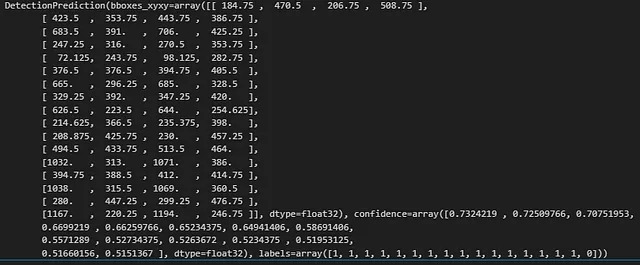
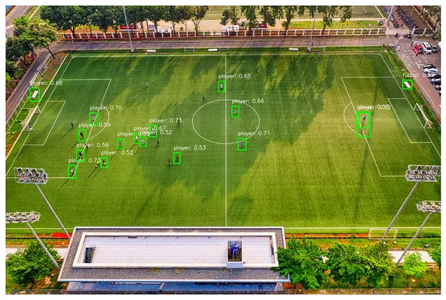
Now display bounding boxes and labels
import cv2
import matplotlib.pyplot as plt

label_dict={0:"player",1:"referree",2:"football"}

# Load the image (replace with your image loading method)
image = cv2.imread(image_path)

# Bounding boxes, labels, confidence, and label dictionary
bboxes = model_result.prediction.bboxes_xyxy
confidences = model_result.prediction.confidence
labels = model_result.prediction.labels

# Draw bounding boxes and labels on the image
for i in range(len(bboxes)):
    bbox = bboxes[i]
    confidence = confidences[i]
    label = labels[i]

    # Coordinates of the bounding box
    x1, y1, x2, y2 = [int(coord) for coord in bbox]

    # Draw the rectangle
    cv2.rectangle(image, (x1, y1), (x2, y2), color=(0, 255, 0), thickness=2)

    # Create label text with confidence
    label_text = f"{label_dict[label]}: {confidence:.2f}"

    # Put the label text above the bounding box
    cv2.putText(image, label_text, (x1, y1 - 10), cv2.FONT_HERSHEY_SIMPLEX,
                fontScale=0.5, color=(255, 255, 255), thickness=1, lineType=cv2.LINE_AA)

# Convert BGR to RGB for displaying in matplotlib
image_rgb = cv2.cvtColor(image, cv2.COLOR_BGR2RGB)

# Display the image using matplotlib
plt.figure(figsize=(10, 10))
plt.imshow(image_rgb)
plt.axis('off')  # Turn off axis
plt.show()
