Physical Address
304 North Cardinal St.
Dorchester Center, MA 02124
Physical Address
304 North Cardinal St.
Dorchester Center, MA 02124
→ Model Training: Step-by-step guide for training custom PyTorch Image Classification models with any dataset.
Okay, now it is time for model training. In the first part of this small series about how to train a custom image classification model with PyTorch, I talked about how to prepare dataset so that it will be ready to train a model.

I always follow 6 steps for image classification model training, and I already covered the first 3 steps in the first part of this small series, you can read it.
Now, it is time for step 4, 5, and 6, which are all about model training. Let’s start !
Also, I have a YouTube video about this article, you can watch it.
To train a model with PyTorch, you need to create your own functions. PyTorch does not provide a function similar to .fit() in Tensorlow. I am going to write 2 function for training the model, one for training, and one for validation.
In these functions:
Function for training set
# add accuracy values to the list
train_accuracies=[]
validation_accuracies=[]

# Function for training
def train(dataloader, model, loss_fn, optimizer, epoch):

    size = len(dataloader.dataset) # total number of images inside of loader
    num_batches = len(dataloader) # number of batches

    model.train()

    train_loss, correct = 0, 0


    for batch, (X, y) in enumerate(dataloader):
        # move X and y to GPU for faster training
        X, y = X.to(device), y.to(device)

        # make prediction
        pred = model(X)
        # calculate loss
        loss = loss_fn(pred, y)

        # Backpropagation
        loss.backward() # compute parameters gradients
        optimizer.step() # update parameters
        optimizer.zero_grad() #  reset the gradients of all parameters

        # Update training loss
        train_loss += loss.item() # item() method extracts the loss’s value as a Python float

        # Calculate training accuracy
        correct += (pred.argmax(1) == y).type(torch.float).sum().item()

    # loss and accuracy
    train_loss = train_loss / num_batches
    accuracy = 100 * correct / size

    # use this accuracy list for plotting accuracy with matplotlib
    train_accuracies.append(accuracy)

    # Print training accuracy and loss at the end of epoch
    print(f" Training Accuracy: {accuracy:.2f}%, Training Loss: {train_loss:.4f}")
Function for validation set
# function for validation
def validation(dataloader, model, loss_fn,t):

    size = len(dataloader.dataset) # total number of images inside of loader
    num_batches = len(dataloader) # number of batches

    validation_loss, correct = 0, 0

    # sets the PyTorch model to evaluation mode, it will disable dropout layer
    model.eval()

    with torch.no_grad(): #  disable gradient calculation
        for X, y in dataloader:

            # move X and y to GPU for faster training
            X, y = X.to(device), y.to(device)
            pred = model(X) # make prediction
            validation_loss += loss_fn(pred, y).item()

            # if prediction is correct add 1 to correct variable.
            correct += (pred.argmax(1) == y).type(torch.float).sum().item()

    # loss and accuracy
    validation_loss /= num_batches
    accuracy = 100 * correct / size

    validation_accuracies.append(accuracy)

    # Print test accuracy and loss at the end of epoch
    print(f" Validation Accuracy: {accuracy:.2f}%, Validation Loss: {validation_loss:.4f}")
These two functions train and validation will be used for training.
In the below code, I have explained the meanings of all the layers, what they do, the output dimensions, and how the model works. I strongly recommend you to read the comment lines.
import torch
# if GPU is available , use it while training
device = "cuda" if torch.cuda.is_available() else "cpu"
device
import torch
import torch.nn as nn

class SimpleCNN(nn.Module):
    def __init__(self, num_classes=9):
        super(SimpleCNN, self).__init__()

        # image size is --> (3,180,180)

        # convolutional layer with 32 filter, input dimension is 3 because image has 3 channels
        self.conv1 = nn.Conv2d(3, 32, kernel_size=3, padding=1)
        # activation function , it introduces to the model , and non-linearity helps to model to learn complex functions .
        self.act1 = nn.ReLU()
        # MaxPool2d reduces size (90,90)
        self.pool1 = nn.MaxPool2d(2)

        self.conv2 = nn.Conv2d(32, 64, kernel_size=3, padding=1)
        self.act2 = nn.ReLU()
        self.pool2 = nn.MaxPool2d(2)  # --> (45,45)

        self.conv3 = nn.Conv2d(64, 128, kernel_size=3, padding=1)
        self.act3 = nn.ReLU()
        self.pool3 = nn.MaxPool2d(2) # --> (22,22)

        # first flatten the channels and then feed them into the fully connected layer. Given the input shape of (128, 22, 22), flattening it results in 128 * 22 * 22.
        self.fc1 = nn.Linear(128 * 22 * 22 , 256)
        self.act4 = nn.ReLU()

        # dropout drops weights randomly, and here %20 of weights are dropped randomly. It helps to prevent overfitting.
        self.dropout=nn.Dropout(p=0.2)

        # The nn.Linear layer with input size 256 and output size 9 represents the output layer of our neural network.
        # Since we have 9 classes, the output of this layer will be passed through a softmax activation function.
        # (error function  internally applies softmax activation ,you dont need to add it to here)
        # This converts the raw outputs into probabilities, representing the likelihood of each class.
        # These probabilities are then used to calculate the error during training
        self.fc2 = nn.Linear(256, 9)


    def forward(self, x):

        # add outputs on top of each layer and return out in the end
        out = self.pool1(self.act1(self.conv1(x)))
        out = self.pool2(self.act2(self.conv2(out)))
        out = self.pool3(self.act3(self.conv3(out)))

        out = out.view(out.size(0), -1)

        out = self.act4(self.fc1(out))
        out=self.dropout(out)
        out=self.fc2(out)

        return out

# create the model
model = SimpleCNN()
model.to(device)

Training might take a long time depending on your GPU.
# Loss funciton and optimizer
loss_fn = nn.CrossEntropyLoss()
optimizer = torch.optim.SGD(model.parameters(), lr=1e-3)
# epoch number
epochs = 32

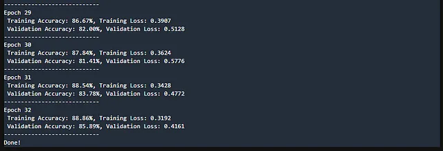
# loop for training model
for t in range(epochs):
    print(f"Epoch {t+1}")
    train(train_set, model, loss_fn, optimizer,t)
    validation(validation_set, model, loss_fn,t)
    print("----------------------------")
print("Done!")

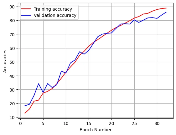
Okay, training is finished. Now, it’s time to make some observations about the model, let’s display the accuracy.
import matplotlib.pyplot as plt

def visualize(train_accuracies,validation_accuracies):
    epoch_number=len(train_accuracies)

    plt.plot(range(1,epoch_number+1),train_accuracies,'r', label='Training accuracy')
    plt.plot(range(1,epoch_number+1),validation_accuracies,'b', label='Validation accuracy')
    plt.legend()
    plt.xlabel("Epoch Number")
    plt.ylabel("Accuracies")
    plt.grid()


# Remember, train_accuracies and validation_accuracies are lists, they stored accuracy values while training
visualize(train_accuracies,validation_accuracies)
