Physical Address
304 North Cardinal St.
Dorchester Center, MA 02124
Physical Address
304 North Cardinal St.
Dorchester Center, MA 02124
→ A step-by-step guide to training image classification models using TensorFlow Keras with any custom dataset.
I wrote 2 articles about training image classification models in PyTorch, and it is now time for Keras. In this article, I will cover dataset creation, visualization of the dataset, visualization of class distribution, training an image classification model, and visualization of the model’s training metrics.

Also, I have a YouTube video about this article, you can watch it.
For training any kind of deep learning model, you need to prepare datasets that consist of training and validation sets (you can create a test set as well). You can split them at any rate you prefer. I typically split 70% for the training set and 30% for the validation set.
If you don’t have enough images or if you want to increase the diversity of your dataset, you can use data augmentation. However, if you already have sufficient data, after splitting your dataset into training and validation sets, you can train your model directly with these datasets.
Data augmentation is a technique to increase the diversity of your training set by applying random transformations, such as image rotation, image scaling, and more .
Augmented images are generated from original images with different orientations, scales, brightness levels. Keras provides a very useful function called ImageDataGenerator for the augmentation process.
Augmented datasets are used for prevent overfitting, helping the model generalize better.
Note : Augmentation is applied only to the training set.
from tensorflow.keras.preprocessing.image import ImageDataGenerator

# your directories
training_dir="datasets/training_set"
validation_dir="datasets/validation_set"

# if you want to augmented dat set use it like this : prep_data(True)
def prep_data(augmented,batch_size=16):
    if augmented:
        # you can change this parameters
        train_datagen = ImageDataGenerator(
            rescale=1./255,
            rotation_range=40,
            width_shift_range=0.2,
            height_shift_range=0.2,
            shear_range=0.2,
            zoom_range=0.2,
            horizontal_flip=True)
        # Augmentation is applied only to the training set
        validation_datagen = ImageDataGenerator(rescale=1./255)

    else:
        # if you set augmented=False , images are just rescaled
        train_datagen = ImageDataGenerator(rescale=1.0 / 255.0)
        validation_datagen = ImageDataGenerator(rescale=1.0 / 255.0)

    # training set
    train_set = train_datagen.flow_from_directory(
        training_dir,
        target_size=(180, 180),  # The dimensions to which all images found will be resized
        batch_size=batch_size,#
        class_mode="sparse") # you can change this to onehotEncoded format or another format


    # validation set
    validation_set = validation_datagen.flow_from_directory(
        validation_dir,
        target_size=(180, 180),
        batch_size=batch_size,
        class_mode="sparse")

    return train_set , validation_set

This function returns train and validation datasets, and with these sets you can train and evaluate models .
This step is not really necessary but I think it is good to see some examples from your dataset. Particularly when using an augmented dataset, it is helpful to observe some example augmented images because sometimes the augmentation might not always produce the expected results.
import matplotlib.pyplot as plt

# create dataset (augmented or not augmented , it is up to you , process is same in both cases
train_set,validation_set=prep_data(True)

images,labels=train_set.next()

class_names = train_set.class_indices
class_names = {v: k for k, v in class_names.items()}

fig, axes = plt.subplots(1, 4, figsize=(15, 5))

for i in range(4):
    axes[i].imshow(images[i])
    label_index = int(labels[i])
    class_name = class_names[label_index]
    axes[i].set_title(f"{class_name}")
    axes[i].axis('off')

plt.tight_layout()
plt.show()


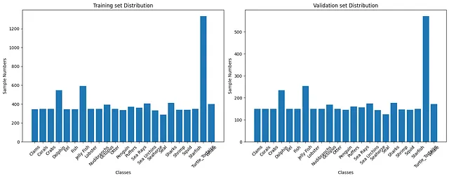
Balancing a dataset is a crucial step because it helps to prevent the model from becoming biased towards one class. If you have an imbalanced dataset, the results may not be satisfactory. Visualizing the distribution can be useful for determining whether the dataset is balanced or imbalanced.
import os
import matplotlib.pyplot as plt

# train an validation folders path
train_dir = "path_to_training_dir"
validation_dir = "path_to_validation_dir"

# calculate distribution in training set
train_class_counts = {}
for class_folder in os.listdir(train_dir):
    class_path = os.path.join(train_dir, class_folder)
    if os.path.isdir(class_path):
        num_images = len(os.listdir(class_path))
        train_class_counts[class_folder] = num_images

# calculate distribution in validation set
validation_class_counts = {}
for class_folder in os.listdir(validation_dir):
    class_path = os.path.join(validation_dir, class_folder)
    if os.path.isdir(class_path):
        num_images = len(os.listdir(class_path))
        validation_class_counts[class_folder] = num_images


plt.figure(figsize=(15, 6))

# training
plt.subplot(1, 2, 1)
plt.bar(train_class_counts.keys(), train_class_counts.values())
plt.title('Training set Distribution')
plt.xlabel('Classes')
plt.ylabel('Sample Numbers')
plt.xticks(rotation=45)

# validation
plt.subplot(1, 2, 2)
plt.bar(validation_class_counts.keys(), validation_class_counts.values())
plt.title('Validation set Distribution')
plt.xlabel('Classes')
plt.ylabel('Sample Numbers')
plt.xticks(rotation=45)

plt.tight_layout()
plt.show()

In this case “Starfish” class has way more example than other classes, and you might want to consider reducing number of images in “Starfish” class.
You can always try different backbones, layer combinations, numbers of filters, and so on. I have already trained many models; you can check this kaggle notebook to see the different models. Now, I will use InceptionV3 as the backbone, fine-tune the model by training the last 15 layers, and add a fully connected layer at the end.
from tensorflow.keras.applications import InceptionV3

base_model = InceptionV3(weights='imagenet',
    include_top=False,
    input_shape=(180, 180, 3))

# Freeze the layers except the last 15 layers
for layer in base_model.layers[:-15]:
    layer.trainable = False

# Create the model
model = Sequential()

# # Add the base model
model.add(base_model)
model.add(layers.Flatten())
model.add(layers.Dense(128, activation='relu'))
model.add(layers.Dropout(0.2))
model.add(layers.Dense(256, activation='relu'))
model.add(layers.Dropout(0.15))
model.add(layers.Dense(23, activation='softmax'))

model.compile(
    loss='sparse_categorical_crossentropy',
    optimizer=tf.keras.optimizers.RMSprop(learning_rate=0.00005),
    metrics=['accuracy']
)

model.summary()
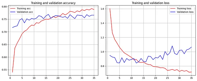
In Keras, the .fit() function is used for training, and if you save it’s output as a variable, it stores the training history of the model.
# you can create train_set and validation_set by following step 1
history = model.fit(
    train_set,
    epochs=35,
    validation_data=validation_set)
By saving this model in some variable(history in above), you can use it for plotting accuracy, loss, or other metrics that you want to visualize.
import matplotlib.pyplot as plt

## visulization function for Models
def visualize(history):
    acc = history.history['accuracy']
    val_acc = history.history['val_accuracy']
    loss = history.history['loss']
    val_loss = history.history['val_loss']
    epochs = range(1, len(acc) + 1)

    fig, axs = plt.subplots(1, 2, figsize=(12, 5))

    axs[0].plot(epochs, acc, 'r', label='Training acc')
    axs[0].plot(epochs, val_acc, 'b', label='Validation acc')
    axs[0].set_title('Training and validation accuracy')
    axs[0].grid(True)
    axs[0].legend()

    axs[1].plot(epochs, loss, 'r', label='Training loss')
    axs[1].plot(epochs, val_loss, 'b', label='Validation loss')
    axs[1].set_title('Training and validation loss')
    axs[1].grid(True)
    axs[1].legend()

    plt.tight_layout()
    plt.show()

visualize(history)
